
Genetic Image: Blueshift (creation)
This describes a little bit about how Blueshift is composed, within the GeneticImage software. I do not describe the process of mutations that created the final product, but rather how the individual pieces make up the whole.
Everything in GeneticImage is composed of functions. A function has a return type (color, number, 2d or 3d vector, or any number of intermediary types), and it may have some number of input types. This forms a tree, with the base of the tree having a color output, and it can branch out quite a bit. Eventually, branches will terminate in either constants or variables that are based on the x and y coordinates of a point. At every point in the image, the tree is evaluated, ultimately producing an image made of colors. Due to the complex nature of the functions, it can sometimes be difficult to understand how images are produced and how the internal functions control the ultimate output.
Here, I have taken the original graph of the functions that define Blueshift, and picked out some of the important branches and made renders of them. I used the “RandomVals$random_v2_col_spline” function to graph functions which return the 2d vector “LVect2d” type, and did something similar with the scalar “LDouble” type, so it was possible to visualize things that are not just colors.
|
|
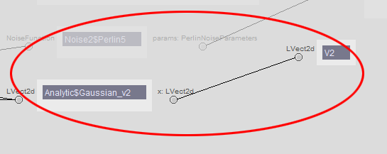
Base01: Genfile, Graph
I chose to pick the base as the simple Analytic$gaussian_v2 of a V2 input. This takes a Gaussian (bell shaped curve) of a 2d vector, making the output into additional bell curves, but in 2d. |
|
|
Base02: Genfile, Graph
The next step creates simple 2d Perlin noise, using the gaussian above as input. This uses the Noise1$noise_v2_v2 function, which takes a 2d vector and produces 2d noise out of it. Because the noise is applied to the squashed gaussian, which has a relatively rapid change in the middle and then much more gradual change the further from the center, the noise has a smooth and wavy feel. |
|
|
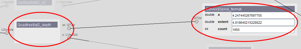
Base03a: Genfile, Graph
This is a quadtree result of a Fermat spiral. The Fermat spiral, as with all of the strange attractor functions, cannot be rendered in 2d using ordinary function evaluation. Instead, it must be evaluated before the computation of the image begins, and the function may simply access the data that was the result of the calculation. Here, data is stored using a quadtree. In this case, we view the quadtree as simply a function which takes a 2d point, projects that point into the space of the quadtree, and returns the depth of the tree reached by the point. If the 2d point has reached maximum depth, then that means that there is a point from the original curve in the quadtree cell. The function returns the depth of the tree that is reached, so it will return 0 if the point is outside the tree, and 1 if the maximum depth is reached. |
|
|
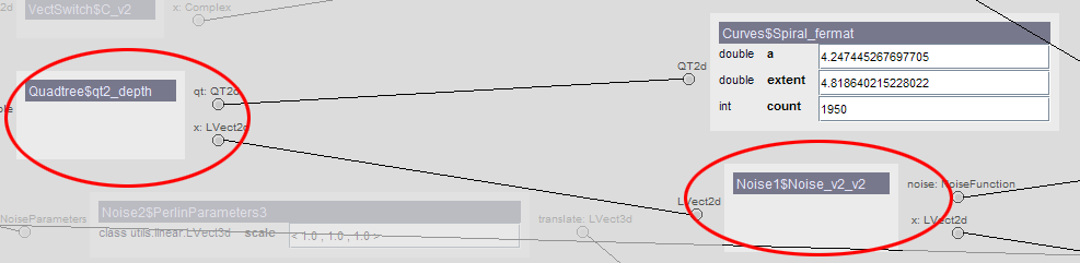
Base03: Genfile, Graph
Now, instead of being evaluated at normal 2d coordinates, the quadtree function is actually evaluated at the result of Base02. This makes the smooth and gradual shading turn into clear curves. It is possible to see some of the orthogonal shapes in the blueish green shapes in the lower middle of the image. However, largely, the crisp grid-like structure from Base03a is entirely gone. Those grids are still present, but they have been warped and distorted beyond recognition. It is useful to note the locations of some of the spots where the result is lighter- a yellow or blue color, because these regions wind up having some dramatic impacts on the final image. |
|
|
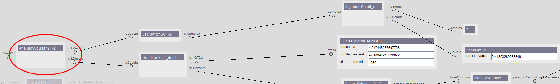
Base04: Genfile, Graph
This now folds the result of evaluating the quadtree back into evaluation of normal vector coordinates. This takes normal 2d coordinates, but applies a squashing function to them, and the amount of the squash is given by the result of Base03. The squashing function is Analytic$Squash2_v2, and where the values of Base03 are high, brings the value of the 2d vector closer to the origin. It still changes slowly over the space of the image, thus contiguous regions have smooth gradients, but those regions still suddenly change at their borders. |
|
|
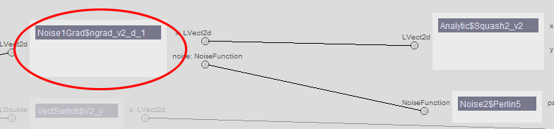
Base05: Genfile, Graph
Here, the result of Base04 is applied to a noise gradient function. The specific function is Noise1Grad$ngrad_v2_d_1, which takes a 2d vector input and produces another 2d vector. The noise gradient functions returns a derivative of the noise based on perturbing the input. The gradient functions are good for creating smooth noise shapes that are different from regular noise. It is a little difficult to articulate how the noise gradient is different, but it includes a directionality that is absent in regular noise. The effect of this yields some rapid changes streaking across the middle of the image, orthogonal to the lines produced by the original curves of Base02. Examining the image closely also reveals some interesting ridge-like curves that appear in the these lines, and these become recognizable features later. |
|
|
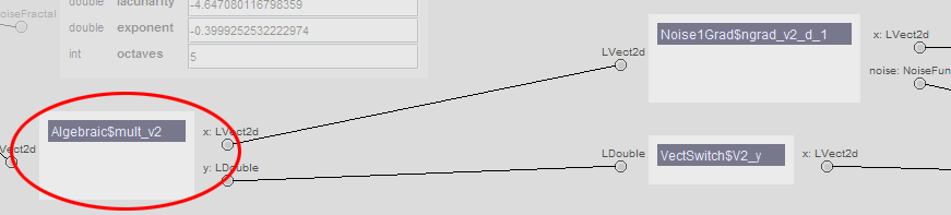
Base06: Genfile, Graph
The noise gradient is then multiplied by another number, the value of which is the y component of the gaussian in Base01. Thus, the values produced by the gradient are significantly scaled down as the y coordinate of a pixel moves above or below the center line. Thus, around the horizontal center, the visual complexity is about the same, but it tapers off and becomes less busy around the upper and lower parts of the image. |
|
|
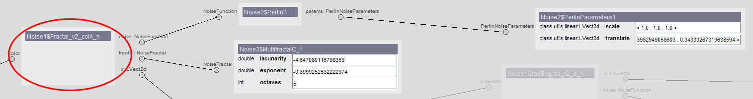
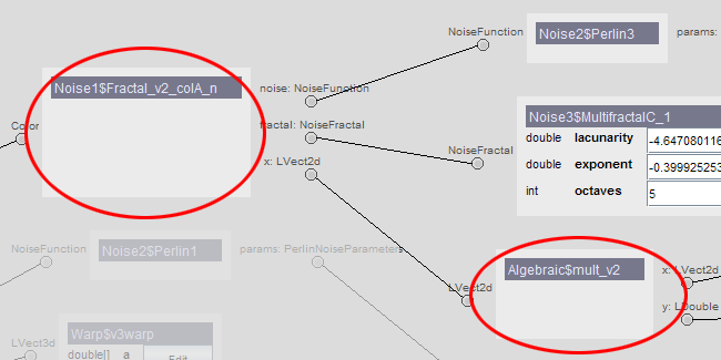
Base07: Genfile, Graph
This is a totally different part of the underlying function graph. This shows a Noise1$Fractal_v2_colA_n function evaluated just on the 2d plane. This particular image uses a multifractal, which produces the rich and visually busy information. Multifractals tend to get lots of folds and warps. Here, the red, green, and blue values are rather dissociated, with green exhibiting the most folding, but the blue and red are just blotches. |
|
|
Base08: Genfile, Graph
Finally, the actual image begins to take shape. Here, instead of seeing the multifractal applied to ordinary 2d space, it is applied to the result of Base06. The resulting image is still very much stark contrasts of red, green, and blue, but we begin to see some interesting layering and folding appear in each of the colors. The regions and features from Base06 become much more pronounced and visible. Instead of seeing the features as regions of gradual or rapid change, here they become actual regions of color. |
|
|
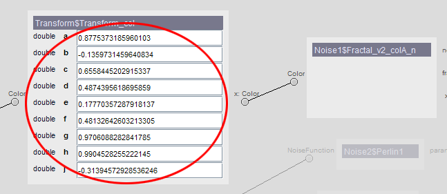
Base09: Genfile, Graph
Now, the image begins to look more like the final product. This is a point at which I intervened in the process of creating the image. Having worked with image generation for so long, I have become very frustrated by the predominance of the primary red, green, and blue colors. There is nothing wrong with these colors, but very often they are aligned as channels to different channels of information, and this is a tedious use of the color spectrum. Here, I created a Transform$Transform_col which wound up mapping the green to blue, red to mauve, and blue to a yellow. The result is very dark, but does create areas of strong contrast between light and dark regions. |
|
|
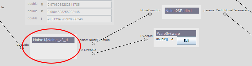
Base10: Genfile, Graph
Another branch of the function tree produces a simple 1 dimensional noise. This is applied to a warped 3 dimensional vector, creating a distribution that stretches across the image. I believe that the pink regions in this image have a higher value, while the green regions have a lower value. |
|
|
Final: Genfile, Graph
The final version takes Base09 and applies a ColorOp$Blend_to_White function to it, taking the second argument, the blend amount, as the result of Base10. What this does is that it takes the original color and mixes in an amount of white equal to the blend amount. The values appear to be fairly low, as there is very little pure white, but this also manages to lighten the original image as well. The nice thing about this function is that in addition to lightening the colors, it also softens them. Base09 was much more balanced than Base08, but it was still very heavy on the primaries. There were fewer grays and soft tones. Here, large portions of the image have been softened so that the color is not as severe. |


